This is a post describing fae¹, a project I worked on in late 2024 as part of TPU Research Cloud. It is a library for training sparse autoencoders² and is behind "Interpreting Large Text-to-Image Diffusion Models with Dictionary Learning".

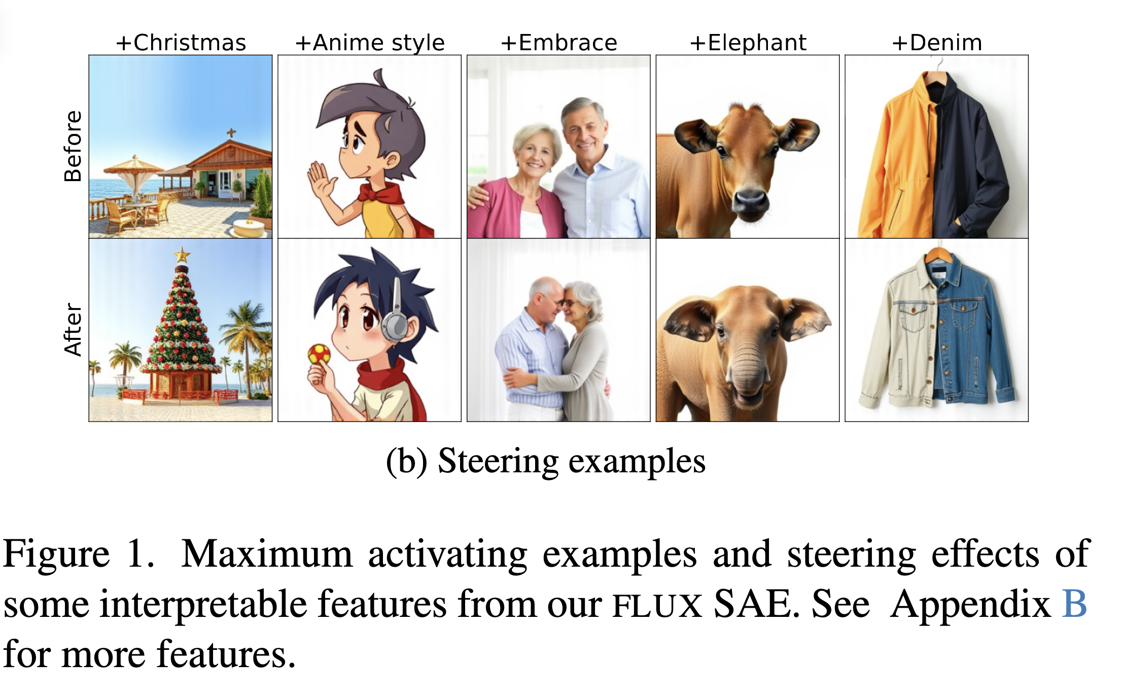
Code: http://github.com/neverix/fae.

FLUX implementation

FLUX.1 came out in August 2024. It is a MMDiT, like Stable Diffusion 3, which was SOTA at the time. It was quickly adopted and optimized for GPUs. Still, in the next few months, no open source implementation for TPUs came out.

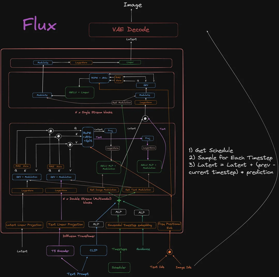
I requested TPUs from TRC to port this model to TPUs and got access to v4-8 and v3-8 TPUs for testing. FLUX was a fairly large model compared to what was out there, with 12 billion diffusion transformer parameters, so quantized versions were published. v4-8 TPUs have 32GB of HBM per chip, meaning that, if one were to use data parallelism, the parameters would just barely fit in bfloat16. For this reason, I considered ways to reduce memory use early into the project. I settled on a combination of FSDP and 4-bit quantization. In the end, I had a reasonably efficient FLUX.1 runtime capable of generating images and suitable for SAE training.

Memory use optimization: FSDP

As mentioned above, each v4 TPU chip has 32GB of RAM. However, there are 4 of them linked on a v4-8 node, so the actual memory we're working with is the combined 128GB. Normally, this would mean we have to use a sharding strategy like pipeline or tensor parallelism instead of using different the different chips for different data elements, meaning we probably have to eat a performance penalty because the sizes of the matrix multiplies aren't maximized

But because the TPUs have very fast interconnect we can use a strategy like FSDP that shards parameters but doesn't actually split the computation together with them. The simplest way to make FSDP work is similar to torch's FSDP2: shard each parameter across one arbitrary axis, gather them for the matmul, and perform a matmul with data local to each node.

This is pretty easy to do in Jax: we can just add an FSDP axis to each of the parameters when specifying the sharding to send the model to. We use the last (output) axis for each 2D parameter and don't shard 1D parameters.

Now, to actually use the parameters, we have two options. Either each linear layer takes its sharded and unshards it before doing its computation (with rematerialization, obviously), like in torch's FSDP, or we need to write a custom matmul using shard_map. I went the latter route, thinking it was necessary for matmul with FSDP work; as it turns out, as long as the batch is sharded as "fsdp None None" and the weight as None fsdp, XLA implements the torch FSDP "unshard-then-matmul" method automatically. While this is negligibly less memory-efficient, it actually wins out on speed for larger batch sizes, so opting to write a custom matmul for FSDP was a bad idea in retrospect.

Memory use optimization: 4-bit quantization

Flux doesn't inference with bfloat16 activations by default; some components (TODO look up which) need to be computed in float32 for generations to not explode. However, its parameters are pretty robust to quantization; it is regularly inferenced in fp8, and normalfloat4 from bitsandbytes works well enough for the community to use it.

This quantization method is similar to the int8 quantization commonly used for language models with bitsandbytes. These methods take a 2D weight matrix, then normalizes it to range from 0 to 1. Then, the rescaled values are assigned to one of a few discrete quantization bins for compression. As the original paper points out, weights of LLMs usually have outliers, with outliers corresponding to either specific rows or specific elements. For this reason, the most commonly used normalization starts by normalizing each row (dividing it by its maximum value and storing a per-row factor), which means an outlier in any given row only increases quantization error by increasing scale only in that row, and then, for each row, taking blocks of 32-128 elements and similarly normalizing each block by its scale (or scale and offset) -- picking blocks of elements is the simplest possible noisy heuristic for splitting up elements in such a way that any single element being an outlier doesn't affect the others.

NF4 quantization is similar to FP8 and distinct from the original int8 in that, after normalizing the weights this way and storing normalization factors in bfloat16,

We wrote a Pallas kernel which works with 4-bit quantized weights directly. It loads chunks of the inputs and weights into vector memory (SRAM), dequantizes them inside vector memory, and performs matrix multiplication the same way the default matmul. There were a lot of restrictions on v4-8's that prohibited more complicated quantization schemes or ones that actually improve efficiency (see below), and we ran into open compiler bugs.

However, at least on v4-8's, this kernel is unnecessary. Because the TPU is incapable of performing lower-precision operations, it still needs to do a bfloat16 matrix multiplication with the loaded parameters. The only efficiency improvements it could offer are on memory bandwidth. TPUs normally achieve very high MFU on matrix multiplication, and indeed, eager dequantization is just as fast as a custom kernel on v4-8 devices. There may be a way to run faster by using int8 quantization and quantizing individual rows and columns and square blocks instead of per-row blocks, so that the matmul itself can be done in int8 on blocks of elements which all have the same scale, but this is only possible on v5 TPUs, which we didn't have access to at the time.

The quantization happens entirely on the CPU while the model is being loaded for the first time, along with separating QKV projections and converting into a layer-sliced format (see below).

In practice, to store the weights in a quantized format, we create a custom tensor class with qax and define a few operations for it such as concatenation and slicing (for the optimization below), along with the matrix multiplication described previously. In practice, this approach is prone to bugs, and, given there aren't that many operations that are done on all weights of a network, it would be easier to use a custom wrapper which treats quantized tensors as leaves and maps over them for each of those. We call this format MockQuantMatrix and use it in practice instead of the qax method.

One specific limitation quantization imposes is that the batch dimension must be propagated exactly through the network so the kernel can see the right batch shape when optimizing; this means we cannot use vmap at any point in the hierarchy, even though Equinox (the jax framework we used) strongly encourages this. A consequence of this is that we needed to define versions of the framework's primitives that automatically batch, like VLinear and VLayerNorm. This entire problem may be solvable with a custom vmap rule.

Layer slicing

The other big hurdle other than memory use is compilation time: jax can take minutes to compile large models, with compile time scaling linearly with the number of operations -- or, equivalently for neural networks, the number of layers.

A possible way to fix this is to reshape the network's parameters so there is only ever one single layer in the model definition, but that layer's parameters have a preceding layer dimension; then, at runtime, we use a scan (or for loop) to iterate over values of the tensor and run one single compiled implementation. This means we only need to pay the cost of compiling the forward and backward pass of one layer, and is only possible because in modern transformers the operations executed in each layer are exactly the same.

In practice, this is implemented as an equinox module with special handling for regular quantized tensors and the dataclass-wrapped version described in the last paragraph of the previous section. The tensors concatenated across layers are created on CPU and sent straight to the correct sharding on TPU, so at runtime this is always efficient.

The layer sliced sequential scan approach creates some unique challenges for interpretability, which requires capturing activations, which will be described below.

T5

Like Imagen and its successors, FLUX 1 has frozen two text encoders: the CLIP text encoder and T5 11B. The format is relatively straightforward to implement, as the network is small enough to not need special optimization and is already implemented in Huggingface's (now deprecated) Flax API.

T5 has several implementations; t5x and the Huggingface one are notable, but the former had too complicated of an interface. We use the Huggingface implementation, but because the model has so many parameters, it needs the extra optimizations -- namely, FSDP for large parameters and enabling an arbitrary number of batch axes (including none) in all of the modules. We implement these, along with custom linear layers for quantized matmul and disabling caching and the decoder head. We also separate out only the 5.5B parameter encoder and quantize its parameters beforehand in a separate conversion step.

VAE

Flux is a latent diffusion model, so we need a VAE to decode images. The Flux VAE didn't have a Jax implementation, and its architecture is pretty complex, requiring attention; however, madebyollin released a smaller network that is a stand-in replacement for Flux can approximately encode and decode from Flux's latent space with only convolutions. I just needed to port this model to Jax.

The approach I took is somewhat roundabout. I converted this network into ONNX (notebook) with a batch size of one and an arbitrary resolution. Jax has an ONNX runtime, which I could use to turn the network into a Jax function and then vmap it for execution, but it doesn't support the model by default. As seen in the notebook, as a replacement, I considered using tensorflow's ONNX runtime and then converting the tensorflow function into Jax. What I ended up doing was creating a fork of the Jax ONNX runtime (shortened to jort in the repository) with a minimal implementation of the missing function necessary to run the model, Resize.

SAE training

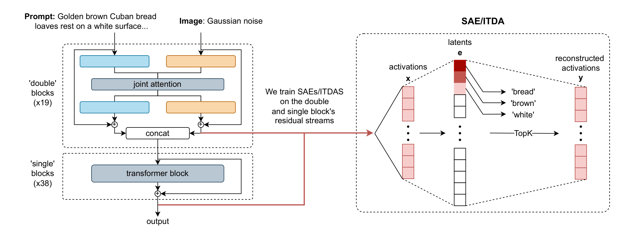
We train SAEs on residual stream activations of the transformer on image tokens. Flux has 19 two-stream blocks, where text and images have separate linear parameters but otherwise the same residual stream, and 38 single-stream blocks where both image and text tokens are treated the same way. We train SAEs on the boundary between the two, as that's exactly halfway through the model in terms of parameters.

We train on Flux Schnell, the timestep-distilled variant of Flux which can generate images in one step; we use a trick to generate the data without storing images on the TPU's limited SSD: we only feed in noise and generate images in one timestep to produce the latents we train on. This seems to produce reasonable results. To generate the images, we use prompts from CC12m. We trained with more timesteps (4) with a similar data source (sampled images) but didn't evaluate those runs.

We train TopK SAEs with an L0 of 64 and 16k features. Initially, training these SAEs failed -- variance explained didn't decrease quickly, and many features were dead or activated infrequently. We looked at a PCA of the mid-layer activations we were training on, and found they had very low effective rank,³ with only a dozen dimensions explaining much of the variance. We found that normalizing the data by either rescaling each column or performing PCA on it before training fixed the problem of latents dying and produced reasonable activation dashboards.

SAE training details

We train k=64 SAEs with 65536 features on the last layer of Flux's double blocks. We perform the aforementioned whitening to the training data. For preventing dead features, we use gradint clipping and a variant of ghost gradients (or AuxK) which picks dead features and tries to reconstruct the output with them, though it doesn't help much. We log weight and gradient norms and otherwise train with no-momentum Adam.

We partition the SAE with tensor parallelism and use Jax's distributed approximate TopK. orbax's checkpointing is used for training (and also all other e.g. quantized model saving). We create activation buffers on CPU every 16 batches of 4 images, where we shuffle the data and prepare it for asynchronously transferring back.

We store activation dashboards in a numpy array which records for each image a variable number of possible activating features along with a variable number of activating positions for improved efficiency over storing all top-k activations on each image token. We additionally store a priority queue of top image activations per feature. We use numba on mmap'd arrays for efficiency.

Sparse operations on TPUs

SAEs naturally perform a sparse matrix multiplication in the decoder; on GPUs, properly implementing it to take advantage can speed up training 6x by removing almost half of the FLOPs for the forward pass and almost all the FLOPs for the backward pass (see Gao et al. 2024 (Section D)). This shifts the bottleneck rightly into memory bandwidth (see https://www.neuronpedia.org/graph/info#appendix-e).

TPUs do offer a way to write kernels through Pallas, but the language isn't expressive enough for sparse matrix multiplication. While it is possible to write a kernel that uses the scalar shared memory of the TPU, we can't express a matmul that is more efficient than the baseline. While writing this, I also benchmarked SparseCores, which TPU v5 and up expose as an API for performing sparse operations for recommendation systems. As expected, at least on v5-8 they did not help with speed enough to outperform the baseline:

def get_smatmul_fn(W):
    def sparse_matmul_basic(wi):
        weights, indices = wi
        return (weights[:, None] * W[indices]).sum(0)
    return sparse_matmul_basic

SPARSE_MATMUL_MAX_BATCH = 32768
@jax.remat
def sparse_matmul_scan(
    weights: Float[Array, "batch_size k"],
    indices: UInt[Array, "batch_size k"],
    W: Float[Array, "n_features d_model"]) -> Float[Array, "batch_size d_model"]:
    return jax.lax.map(get_smatmul_fn(W), (weights, indices),
                       batch_size=SPARSE_MATMUL_MAX_BATCH // weights.shape[-1])

Other methods

In the paper, we compare the trained SAE features to neurons on an interpretability metric (Figure 7). SAE features win on this metric, but I'm pretty skeptical of the result now. The metric involves taking the max-activating examples for individual features (from SAEs or neurons), asking a VLM to describe them, and then, based on the description, classifying whether a specific image came from this neuron's max-activations or from another neuron's, with higher scores meaning better interpretability.

We train an SAE with 65,536 features, which is somewhat larger than to 12,288 neurons in the MLPs. At a glance, max activations of both neurons and SAEs are interpretable; however, MLP neurons underperform on our automated interpretability eval. This may be a sign there is something wrong with the eval, as we didn't check it very thoroughly. I would expect MLP neurons to be comparable in terms of representing concepts compared to transcoders, but perhaps SAEs can split the features up to a greater extent.

I discovered fluxlens, another project which trains SAEs on FLUX, while writing this blog post. Their architecture is pretty similar to what we do, but without normalization, so I'm surprised the SAEs don't have many dead features. Their visualization is pretty well-made and can even visualize individual data points, but it only shows two images per feature without overlaid activation patterns, which can make it hard to tell what a feature is doing, even if it is interpretable. Additionally, it seems their SAEs have 3072 features, which is the d_model of Flux and means they're probably not resolving sperposition and are not much better than a PCA over the data.

Gathering activations

To collect data, need to gather activations from the model's forward pass. This is a problem with Jax, where each function must be pure and we cannot easily change what a function outputs. The most common existing solution is to accumulate the state into a dict that is propagated up the tree -- for example, in penzai v1, used in saex. flax nnx instead stores the intermediates as state attached to the module object and then collects it. flax linen works around the restrictions on mutability by creating a global thread-local context which capture of intermediates stores.

All three of these solutions require scaffolding and a somewhat heavy framework, which aren't feasible in Equinox, which I implemented this in. I experimented with passing captured intermediate values as a second output, but it seemed deeply suboptimal.

The other solution is Harvest's sow and reap. They create a custom interpreter (akin to jax's built-in vmap) which plants values with a tag in the interpreter's state and then pulls them out when a matching reap call is found. This is obviously very convenient for collecting activations that may not be explicitly returned from the model; storing or injecting activations at any given point only requires adding one line of code.

This API has some non-obvious interactions with Equinox that require using Equinox's checkpointed scan. The FluxInferencer, which is used by FluxEnsemble to run the actual model, also supports reaping only from specific layers with a static input change, something which is useful for SAE training.

In the end, this feature required some hacky scaffolding: we have a global Reaper variable which keeps track of which layers' outputs should be recorded for a specific block type, stores those layers' outputs in a fixed-size array (because flax's support for collecting activations inside a layer-scan only allows for unfiltered collection), and then reaps them from that reaper's specific tag. In principle, this could be done with something more similar to Flax's TLS, especially with a stack of Reaper contexts that is dynamically populated based on which model is being run.